Modelling COVID-19 infection across England
In this tutorial we’ll cover some of the work we did as part of our study into fitting a Bayesian spatio-temporal model to predict the COVID-19 infection rate across England.
Study aim and data description
The COVID-19 pandemic has had a profound impact on global health and economies, with the spread and evolution of the virus becoming a major concern for health authorities and policymakers. In this study, we aim to investigate the spread and evolution of COVID-19 occurrences across England. The aim of the study is two-fold: on the one hand, fitting a Bayesian spatio-temporal model to predict the COVID-19 infection rate across mainland England over space and time; on the other hand, investigating the impacts of socioeconomic, demographic and environmental factors on COVID-19 infection.
The first thing is to load all the packages used in the COVID-19 case study.
The study region is mainland England, which is partitioned into 6789
neighbourhoods at the Middle Layer Super Output Area (MSOA) scale. The
shapefile of the study region shape is a
SpatialPolygonsDataFrame, which is used to map the data. It
stores the location, shape and attributes of geographic features for the
neighbourhoods.load
We first load INLA and then retrieve the data from the fdmr example
data store. We’ll use retrieve_tutorial_data to do
this.
library(INLA)## Loading required package: Matrix## This is INLA_25.02.10 built 2025-02-09 19:59:04 UTC.
## - See www.r-inla.org/contact-us for how to get help.
## - List available models/likelihoods/etc with inla.list.models()
## - Use inla.doc(<NAME>) to access documentation
fdmr::retrieve_tutorial_data(dataset = "covid")##
## Tutorial data extracted to /tmp/RtmpbEnKF9/fdmr/tutorial_data/covidNext we’ll use the load_tutorial_data function to load
in the spatial data we want.
sp_data <- fdmr::load_tutorial_data(dataset = "covid", filename = "spatial_data.rds")Now we make a map of the study region
sp_data@data$mapp <- 0## Loading required package: sp
domain <- sp_data@data$mapp
fdmr::plot_map(polygon_data = sp_data, domain = domain, add_scale_bar = TRUE, polygon_fill_opacity = 0.5, palette = "YlOrRd")A map of the study region.
The COVID-19 data and the related covariate information are included in our tutorial data package. We’ll load in the data using same process we used above.
covid19_data <- fdmr::load_tutorial_data(dataset = "covid", filename = "covid19_data.rds")Then the first 6 rows of the data set can be viewed using the following code
utils::head(covid19_data)## MSOA11CD date week LONG LAT cases Population IMD
## 6521 E02006663 2020-03-07 1 -1.77072 51.17063 3 12605 12.94
## 2101 E02002160 2020-03-14 2 -2.07682 52.59541 4 7481 24.79
## 3321 E02003411 2020-03-14 2 -0.57737 51.52327 8 11443 25.13
## 4008 E02004108 2020-03-14 2 -1.43761 53.29906 4 7514 17.33
## 3334 E02003424 2020-03-14 2 -0.71324 51.51317 4 8947 4.58
## 2094 E02002153 2020-03-14 2 -2.05805 52.61565 3 7217 31.88
## carebeds.ratio AandETRUE perc.chinese perc.indian perc.bangladeshi
## 6521 0.01630534 0 0.2153846 0.5384615 0.02307692
## 2101 0.01440074 0 0.4223307 18.2922001 0.11878052
## 3321 0.01265956 1 0.2399232 16.6826615 0.67178503
## 4008 0.02191863 0 0.1455411 0.2910823 0.10584811
## 3334 0.02194874 0 1.3427866 10.4952197 0.21484585
## 2094 0.00000000 0 0.2005884 2.6343942 0.05349024
## perc.pakistani perc.ba perc.bc perc.wb age1 age2 age3
## 6521 0.0000000 1.2307692 0.35384615 89.54615 11.685839 21.01547 27.10829
## 2101 0.5807048 1.7949056 1.82130131 63.15164 13.848416 19.51611 25.77196
## 3321 30.8941139 4.2226488 1.44753679 17.99424 14.812549 23.80495 21.34056
## 4008 0.2778513 0.1984652 0.07938608 94.98545 11.738089 16.34283 28.81288
## 3334 4.0068751 1.0849715 0.40820711 61.38146 9.701576 20.73321 27.51760
## 2094 0.1337256 1.2035304 1.39074619 87.79085 13.759180 16.95996 27.24124
## age4 pm25 no2
## 6521 16.92979 6.608217 5.957610
## 2101 17.99225 8.066084 14.479405
## 3321 11.13344 8.308508 14.164620
## 4008 24.12829 6.813326 8.356319
## 3334 22.68917 7.822982 11.810846
## 2094 21.53249 7.715645 12.522200The response variable in this study is the weekly reported number of COVID-19 cases in each of the 6789 neighbourhoods in main England over the period from 2020-03-07 to 2022-03-26.
Each week is defined to range from Saturday to Friday. Variable
date indicates the start date of each observation week and
variable week indicates the week number that the data are
collected from. Therefore, the time frame of our study is from the week
beginning March 7, 2020 to the week beginning March 26, 2022 inclusive,
which spans 108 weeks. Variables LONG and LAT
indicate the longitude and latitude for each neighbourhood.
We plot the weekly number of reported COVID-19 cases spanning the 108 weeks:
breaks_vec <- c(seq(as.Date("2020-03-07"),
as.Date("2022-03-26"),
by = "3 week"
), as.Date("2022-03-26"))
cases_week <- dplyr::group_by(covid19_data, date) %>% dplyr::summarize(cases = sum(cases))
fdmr::plot_barchart(data = cases_week, x = cases_week$date, y = cases_week$cases, breaks = breaks_vec, x_label = "Date", y_label = "Number of cases")
The weekly reported number of COVID cases between March 7, 2020 and March 26, 2022.
A number of studies have linked different socioeconomic, demographic and environmental factors to explain the variation in COVID-19 infection rates across space (Sun, Hu, and Xie (2021), Choi et al. (2021), Akinwumiju et al. (2022), Al Kindi et al. (2021), Kim et al. (2021), Wang et al. (2020), Berg, Present, and Richardson (2021)). Based on the past studies and data availability, we selected a set of potential socioeconomic, demographic and environmental variables for our model. These covariate data were collected for each MSOA in England, and can be accessed at https://www.nomisweb.co.uk/census/2021/bulk and https://uk-air.defra.gov.uk/data/pcm-data. We also considered two other covariates related to health care for possible inclusion in the model, because existing studies have shown that they may affect infection rates of COVID-19 (Harris and Brunsdon (2021), Lee et al. (2022)). Table 1 provides the full descriptions of the variables.
| Covariate | Full description |
|---|---|
| IMD | Index of multiple deprivation score for how deprived the area is. A lower index indicates a higher level of deprivation. |
| Care home beds | The number of care home beds per adult population |
| Accident and Emergency | There is a hospital that has emergency facilities or not |
| Percentage of Chinese (%) | Percentage of people who are Chinese descent |
| Percentage of Indian (%) | Percentage of people who are Indian descent |
| Percentage of Pakistani (%) | Percentage of people who are Pakistani descent |
| Percentage of Bangladeshis (%) | Percentage of people who are Bangladeshis descent |
| Percentage of African (%) | Percentage of people who are African |
| Percentage of Caribbean (%) | Percentage of people who are Caribbean descent |
| Percentage of white British (%) | Percentage of people who are white British |
| Age 18-29 (%) | Percentage of the adult population who aged 18-29 |
| Age 30-44 (%) | Percentage of the adult population who aged 30-44 |
| Age 45-64 (%) | Percentage of the adult population who aged 45-64 |
| Age >=65 (%) | Percentage of the adult population who aged 65 and over |
| () | Annual mean concentrations of fine particulate matter |
| () | Annual mean concentrations of nitrogen dioxide |
Model specification
We use a Bayesian hierarchical model to predict the spatio-temporal COVID-19 infection rate at the neighbourhood level in England. Let denotes the weekly number of reported COVID cases for neighbourhood and week and denotes the (official) estimated population living in neighbourhood and week . Note that in our data the population size for each neighbourhood is obtained from the 2021 census and does not change over time, i.e., for all . is assumed to have a Poisson distribution with parameters (, ), where is the true unobserved COVID-19 infection rate / risk in neighbourhood and week . We follow a standard path in modelling with a log link to the Poisson and start with a model where the linear predictor decomposes additively into a set of covariates and a Gaussian latent process characterizing the infection of the disease after the covariate effects have been accounted for. The proposed model is given by
A vector of covariates (if needed) is given by for neighbourhood and time period . is a vector of regression parameters. is a spatio-temporal random effect at location and time , which is modelled by
Here follows a stationary distribution of a first-order autoregressive process (AR(1)) and is the temporal dependence parameter that takes on a value in the interval [-1,1], with indicating strong temporal dependence (a first-order random walk), while corresponds to independence across time. is a spatial random effect that is assumed to arise from a multivariate normal distribution. Each follows a zero-mean Gaussian field which is assumed to be temporally independent but spatially dependent at each time period with Matérn covariance function given by
where is the modified Bessel function of second kind, and is the Gamma function. The Matérn covariance function has three hyperparameters:
- controls the marginal variance of the process S(i,t).
- controls the spatial correlation range, which can be defined as .
- controls the smoothness, where higher values leads to processes that are more smoother.
The model is implemented through the INLA-SPDE approach in R programming. A few steps are needed before fitting the model:
- Create a triangulated mesh of the study region
- Build the SPDE model based on the mesh and set priors for the spatial parameters
- Define how the process evolves over time and set prior for the temporal parameter
- Define the model formula
Mesh construction
To implement the SPDE approach, it is necessary to discretize the space by creating a triangulated mesh that establishes a set of artificial neighbors across the study region (i.e., mainland England). This allows for the calculation of spatial autocorrelation between observations. The construction of the mesh has an impact on the model inferences and predictions. Therefore, it is crucial to develop a good mesh to ensure that the results are not overly sensitive to the mesh. Although the construction of the mesh varies depending on the case study, there are some guidelines available to produce an optimal mesh. In this vignette we will construct a two-dimensional mesh using the fmesher::fm_mesh_2d_inla() function. The locations of all neighbourhoods are passed to the function argument “loc” as initial mesh nodes, and then other arguments in the function are tuned to adjust the shape and resolution of the mesh as necessary.
Argument “max.edge” determines the maximum permitted length for a triangle (lower values for max.edge result in higher mesh resolution). This argument can take either a scalar value, which controls the triangle edge lengths in the inner domain, or a length-two vector that controls edge lengths both in the inner domain and in the outer extension to avoid the boundary effect. Although there is no standard for setting a correct value for the max.edge, a value for max.edge that is too close to the spatial range (i.e., a low resolution) will complicate the process of fitting a smooth SPDE. Specifically, the Gaussian random field approximation might deviate strongly from the desired Matern structure, and the marginal variance will vary over the domain rather than being constant, which violates the assumption of a stationary Gaussian process. Conversely, if the max.edge value is too small compared to the spatial range (i.e., a high resolution), the mesh will contain an excessive number of vertices, resulting in a more computationally intensive fitting process that may not necessarily yield improved results. A number of research studies have suggested the max.edge value for the inner domain to be between 1/3 to 1/10 times smaller than the spatial range (note that the spatial range parameter in INLA GMRF is the distance at which the correlation drops to about 0.13). Since the spatial range cannot be known until the model has been fitted, an initial guess needs to be made and 1/5 of the spatial domain is often used in practice. Here, we define the argument “max.edge” such that the outer extension has a triangle density two times lower than than the inner domain (i.e., twice the triangle length for the outer extension edges), so that the original spatial domain is extended without increasing too much computational burden.
Lindgren and Rue (2015) suggested extending the domain of interest by a distance at least equal to the spatial range to avoid the boundary effect. The function argument “offset” specifies the size of the inner and outer extensions around the data locations. In this study, we expand the inner domain by 1/4 of the spatial range initially assumed, and the outer domain by the same amount as the spatial range. In addition, we also use the parameter “cutoff” to avoid building too many small triangles where we have some very close input locations. It defines the minimum allowed distance between observation points. Points with a distance less than the cutoff value will be considered as a single mesh vertex. Here we choose a cutoff value equal to 1/7 of the max.edge value of the inner domain. The mesh for our study region is displayed in Figure @ref(fig:plotmesh), where the blue dots represent the locations of the neighbourhoods.
Here we use the fmesher::fm_mesh_2d_inla to construct
our mesh.
initial_range <- diff(range(sp_data@data[, "LONG"])) / 5
max_edge <- initial_range / 8
mesh <- fmesher::fm_mesh_2d_inla(
loc = sp_data@data[, c("LONG", "LAT")],
max.edge = c(1, 2) * max_edge,
offset = c(initial_range / 4, initial_range),
cutoff = max_edge / 7
)## Warning in fdmr::plot_mesh(mesh = mesh): Cannot read CRS from mesh, assuming
## WGS84Triangulated mesh used to build the SPDE model.
Build the SPDE model on the mesh and set priors for the spatial parameters
We use the INLA::inla.spde2.pcmatern() function to build the SPDE model and specify Penalised Complexity (PC) priors for the parameters of the Matérn field. PC priors for the parameters range and marginal standard deviation of the Matérn field are specified by setting the values , , and in the relations that P(spatial range<)= , and P()= . The spatial range of the process is the distance at which the correlation between two values is close to 0.1. In this study we use a prior of P(spatial range<1.480)= 0.5 for the spatial range parameter based on an exploratory variogram analysis. It means that the probability that the spatial range is smaller than 1.480 degrees of latitude (which is equivalent to about 164 kilometers) is 0.5. controls the marginal standard deviation of the process, and is specified a prior of P( >1)= 0.01.
prior_range <- initial_range
spde <- INLA::inla.spde2.pcmatern(
mesh = mesh,
prior.range = c(prior_range, 0.5),
prior.sigma = c(1, 0.01)
)Define how the process evolves over time and set prior for the temporal parameter
The previous step has specified that in each of the time periods the
spatial locations are linked by the SPDE model. Now we assume that
across time the process evolves according to a first order
autoregressive (AR(1)) process. We specify a PC prior for the temporal
autocorrelation parameter
.
The prior is given by rhoprior, which is a PC prior with
P()=0.9.
In order to fit the model, we also need to define a temporal index (must be an integer starting at 1) and the number of discrete time points we want to model.
We will use the function bru() of package
inlabru to fit the model. bru expects the
coordinates of the data, thus we transform covid19_data
data set to a SpatialPointsDataFrame using the function
coordinates() of the sp package.
sp::coordinates(covid19_data) <- c("LONG", "LAT")Define the model formula
In order to fit the spatio-temporal model, a model formula needs to be defined, by including the response in the left-hand side and the fixed and random effects in the right-hand side.
formula <- cases ~ 0 + Intercept(1) + IMD +
carebeds.ratio + AandETRUE +
perc.chinese + perc.indian + perc.bangladeshi + perc.pakistani + perc.ba + perc.bc + perc.wb +
age1 + age2 + age3 + age4 +
pm25 + no2 +
f(
main = coordinates,
model = spde,
group = group_index,
ngroup = n_groups,
control.group = list(
model = "ar1",
hyper = rhoprior
)
)Fit the model
Finally, we fit the spatio-temporal model using spde approach and
AR(1) process by calling the function bru() of the package
inlabru.
NOTE: Since the data size is quite large the memory requirements of this function call are high. We recommend running on a suitable high memory system. In our case it takes about 13 hours to complete.
Results
We can inspect the results by typing summary(inlabru_model),which shows the parameter estimates of the fixed and random effects. The marginal distributions of the hyperparameters can also be obtained as follows.
model_summary <- summary(inlabru_model)
model_summary_fixed <- inlabru_model$summary.fixed
model_hyperparams <- inlabru_model$marginals.hyperparSummary of the parameter estimates of the fixed effects
The model summary is provided in the tutorial data package so we’ll load that now.
NOTE: If you’ve run the full model above you don’t need to load in the files below.
model_summary <- fdmr::load_tutorial_data(dataset = "covid", filename = "model_summary.rds")
model_summary_fixed <- fdmr::load_tutorial_data(dataset = "covid", filename = "model_summary_fixed.rds")
model_hyperparams <- fdmr::load_tutorial_data(dataset = "covid", filename = "model_hyperparams.rds")
print(model_summary_fixed[2:nrow(model_summary_fixed), 1:5])## mean sd 0.025quant 0.5quant
## IMD -0.0005112128 6.255458e-05 -0.0006338175 -0.0005112128
## carebeds.ratio 1.1166330921 4.605568e-02 1.0263656196 1.1166330921
## AandETRUE 0.0049431635 1.615743e-03 0.0017763654 0.0049431635
## perc.chinese -0.0030466982 6.376484e-04 -0.0042964661 -0.0030466982
## perc.indian 0.0024263610 2.034198e-04 0.0020276654 0.0024263610
## perc.bangladeshi 0.0014271369 2.067729e-04 0.0010218694 0.0014271369
## perc.pakistani 0.0023360953 1.877373e-04 0.0019681370 0.0023360953
## perc.ba -0.0039299175 2.873344e-04 -0.0044930825 -0.0039299175
## perc.bc 0.0083423398 5.652759e-04 0.0072344193 0.0083423398
## perc.wb 0.0044153274 1.466510e-04 0.0041278968 0.0044153274
## age1 -0.0038339689 1.729288e-04 -0.0041729031 -0.0038339689
## age2 0.0003332178 2.639185e-04 -0.0001840531 0.0003332178
## age3 0.0024108905 3.152524e-04 0.0017930070 0.0024108905
## age4 -0.0063447620 2.053866e-04 -0.0067473124 -0.0063447620
## pm25 0.0041042717 1.973304e-03 0.0002366660 0.0041042717
## no2 0.0001506359 5.135262e-04 -0.0008558570 0.0001506359
## 0.975quant
## IMD -0.0003886081
## carebeds.ratio 1.2069005647
## AandETRUE 0.0081099616
## perc.chinese -0.0017969304
## perc.indian 0.0028250566
## perc.bangladeshi 0.0018324044
## perc.pakistani 0.0027040536
## perc.ba -0.0033667525
## perc.bc 0.0094502602
## perc.wb 0.0047027580
## age1 -0.0034950347
## age2 0.0008504886
## age3 0.0030287739
## age4 -0.0059422116
## pm25 0.0079718774
## no2 0.0011571288Table 2 reports the regression coefficient values, the estimated relative risks and 95% credible intervals between each covariate and COVID infection from our model. The estimated relative risks and 95% credible intervals are computed by exponentially transforming the regression coefficients associated with the covariates described in Table 1. The relative risks relate to realistic increases in each covariate, which are given in brackets in column 1 of the table.
| Covariate | Regression coefficient | Relative risks (95% CI) |
|---|---|---|
| IMD (10) | -0.0005 | 0.9949 (0.9937, 0.9961) |
| Percentage of Chinese (1) | -0.0030 | 0.9969 (0.9957, 0.9982) |
| Percentage of Indian (1) | 0.0024 | 1.0024 (1.0020, 1.0028) |
| Percentage of Pakistani (1) | 0.0023 | 1.0023 (1.0020, 1.0027) |
| Percentage of Bangladeshis (1) | 0.0014 | 1.0014 (1.0010, 1.0018)) |
| Percentage of African (1) | -0.0039 | 0.9961 (0.9955, 0.9966) |
| Percentage of Caribbean (1) | 0.0083 | 1.0084 (1.0073, 1.0095) |
| Percentage of white British (%) | 0.0044 | 1.0044 (1.0041, 1.0047) |
| Age 18-29 (1) | -0.0038 | 0.9962 (0.9958, 0.9965) |
| Age 30-44 (1) | 0.0003 | 1.0003 (0.9998, 1.0009) |
| Age 45-64 (1) | 0.0024 | 1.0024 (1.0018, 1.0030) |
| Age >=65 (1) | -0.0063 | 0.9937 (0.9932, 0.9941) |
| (1 ) | 0.0041 | 1.0041 (1.0002, 1.0080) |
| (10 ) | 0.0002 | 1.0015 (0.9915, 1.0116) |
| Care home beds (0.01) | 1.1166 | 1.0112 (1.0103, 1.0121) |
| Accident and Emergency (TRUE) | 0.0049 | 1.0050 (1.0018, 1.0081) |
The table shows clear evidence that a high level of socio-economic deprivation is associated with increased COVID-19 incidence. An increase of 10 scores in IMD is significantly associated with a 0.5% decreased infection rate. The number of care home beds per adult is also significantly associated with COVID infection, because if a neighbourhood increases its care home beds ratio by 0.01, the estimated risk increases by around 1.1%. In addition, having a hospital with emergency facilities in a neighbourhood is diagnosed positively and significantly associated with higher infection risk (RR:1.0050, 95% CI: 1.0018-1.0081).
Ethnicity appears overall to have a strong association with COVID-19 infection. Neighbourhoods with a greater percentage of Chinese population have lower risk of infections. However, Indian and Pakistani ethnic groups have been found to have a small detrimental effect of COVID infection, with risk increasing by 0.2% as the percentage of Indian or Pakistani ethnic groups in a neighbourhood increases by 1%. African population is associated with decreased risk of COVID-19 infection (RR:0.9961, 95% CI: 0.9955-0.9966), whereas Caribbean population has statistically higher COVID-19 infections (RR: 1.0084, 95% CI: 1.0073-1.0095). Neighbourhoods with a greater percentage of white British have higher risk of infections, with a 1% increase in the population being associated with a statistically significant 0.4% increase in COVID infection.
In addition, we have also found that infection rate is lower in both neighbourhoods with greater population percentages of adults age 65 years and older (RR: 0.9937, 95% CI: 0.9932–0.9941) and neighbourhoods with greater percentages of adults age 18–29 years (RR: 0.9962, 95% CI: 0.9958–0.9965). In contrast, the population between 30 and 44 years old and the population between 45 and 64 years old are positively associated with risk of infections, although the result for the former is not significant. Finally, elevated concentrations are statistically significantly associated with COVID-19 incidence, with a increase in concentrations being associated with between a 0.02% and a 0.80% increased risk. A increase in concentrations is associated with a positive, but insignificant increase in the relative risk of COVID infections (RR: 1.0015, 95% CI: 0.9915, 1.0116).
Summary of the hyperparameters
The parameter estimates of the spatial range parameter, marginal standard deviation of the latent Gaussian process and the AR(1) coefficient are
model_summary$inla$hyperpar[, 1:5]## mean sd 0.025quant 0.5quant 0.975quant
## Range for f 0.297 0.003 0.291 0.298 0.301
## Stdev for f 0.646 0.003 0.640 0.646 0.651
## GroupRho for f 0.838 0.001 0.835 0.838 0.840To plot the posterior distributions of the spatial range, the standard deviation and temporal dependence parameters of the spatio-temporal random effect, we create a list named list_marginals containing the posterior distributions for each parameter. From this list, we generate a data frame margs, and include an additional column named ‘parameter’ which specifies the name of the corresponding distribution for each parameter. Spatial range is estimated to be 0.297, and AR(1) coefficient is estimated to be 0.839, indicating a high level of temporal dependence.
list_marginals <- list(
"Spatial range" = model_hyperparams$`Range for f`,
"Stdev" = model_hyperparams$`Stdev for f`,
"AR(1)" = model_hyperparams$`GroupRho for f`
)
margs <- data.frame(do.call(rbind, list_marginals))
margs$parameter <- rep(names(list_marginals),
times = sapply(list_marginals, nrow)
)
margs$parameter <-
factor(margs$parameter, levels = c("Spatial range", "Stdev", "AR(1)"))
ggplot2::ggplot(margs, ggplot2::aes(x = x, y = y)) +
ggplot2::geom_line() +
ggplot2::facet_wrap(~parameter, scales = "free") +
ggplot2::labs(x = "", y = "Density") +
ggplot2::theme_bw()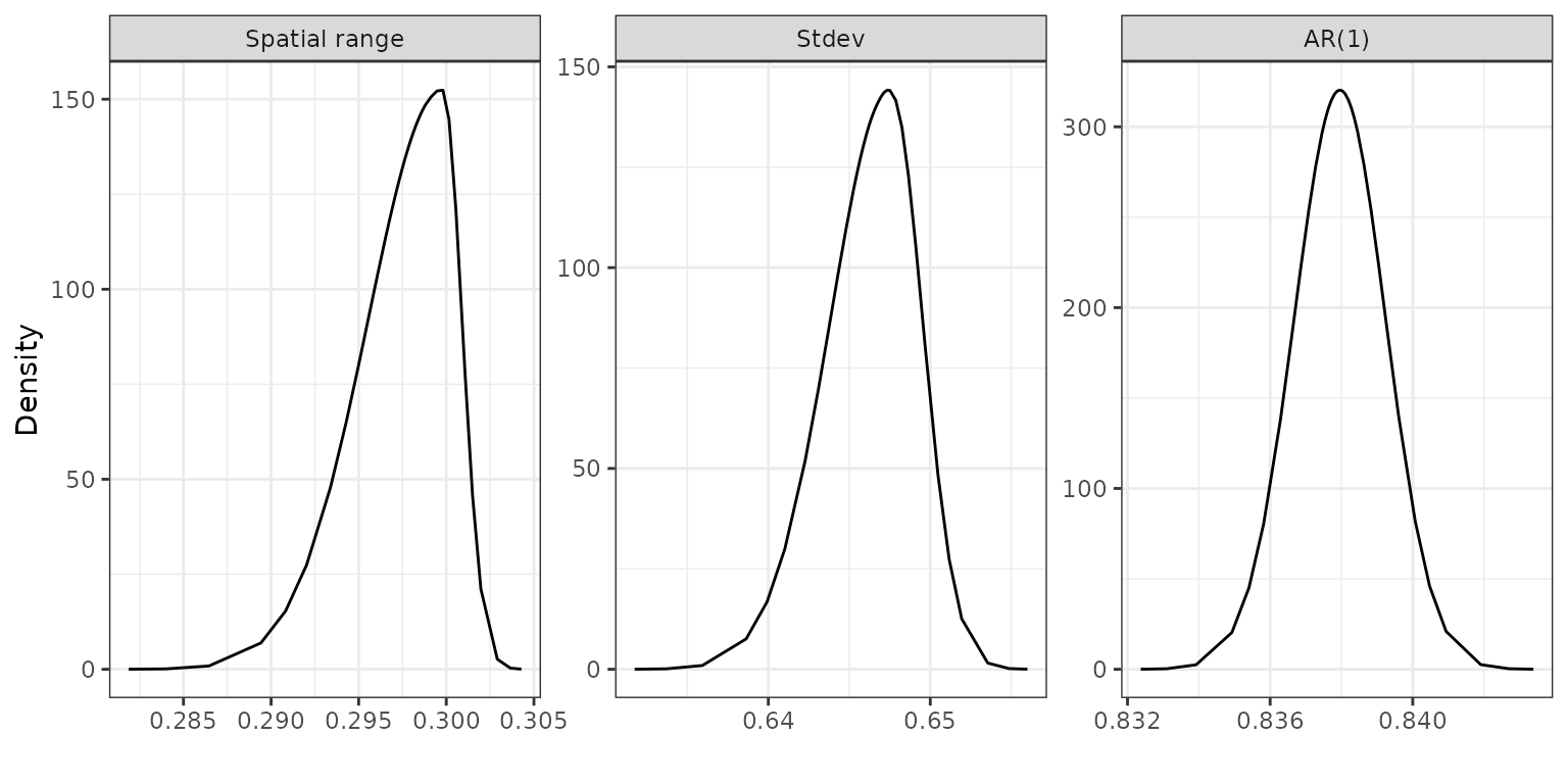
Posterior distributions of the spatial range, standard deviation and temporal dependence parameters.
Temporal evolution of infection rate predictions
The infection rate predictions from the model can be computed using the following codes, and are saved in a data frame called “predictions”.
NOTE: This cell will only run if the model above has been run. Otherwise please run the cell below it which loads in the saved predictions from file.
pred.mean <- inlabru_model$summary.fitted.values$mean[1:nrow(covid19_data)]
pred.25 <- inlabru_model$summary.fitted.values$`0.025quant`[1:nrow(covid19_data)]
pred.975 <- inlabru_model$summary.fitted.values$`0.975quant`[1:nrow(covid19_data)]
predictions <- cbind.data.frame(
"date" = covid19_data$date,
"week" = covid19_data$week,
"MSOA11CD" = covid19_data$MSOA11CD,
"pred.mean" = pred.mean,
"pred.25" = pred.25,
"pred.975" = pred.975
)The date frame “predictions” is provided in the tutorial data package, we’ll load that in now.
predictions <- fdmr::load_tutorial_data(dataset = "covid", filename = "predictions.rds")The figure below displays the boxplots of the predicted infection risk for all neighbourhoods over time. It can be seen that health inequalities in COVID infection exist in England, as there are large differences between the estimated disease risks.
breaks_vec <- c(seq(as.Date("2020-03-07"),
max(predictions$date),
by = "3 week"
), as.Date("2022-03-26"))
fdmr::plot_boxplot(
data = predictions,
x = predictions$date,
y = predictions$pred.mean,
breaks = breaks_vec,
x_label = "Week of date",
y_label = "Infection risk"
)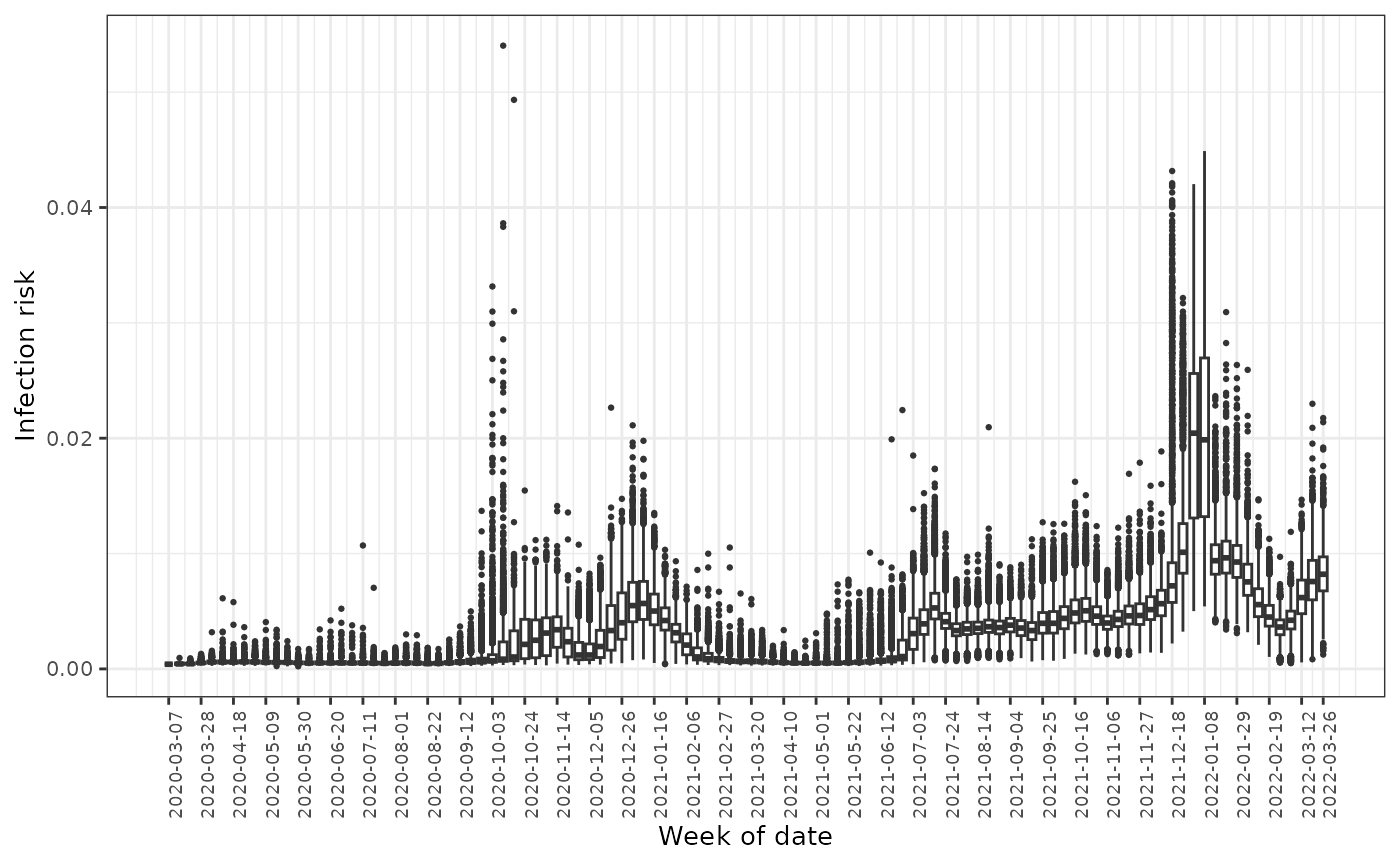
Boxplots of the predicted infection rates across all neighbourhoods over time
The figure below provides the line plot for the average predicted risk with 95% credible intervals by week across England. The COVID infection risk witnessed a series of fluctuations over the study period within the range between 0.0002 and 0.05, while an overall upward temporal trend can be observed. There was an initial peak in mid-November 2020, after which the infection levels declined before rising again in mid-December 2020, which were driven by the emergence of the Alpha variant and peaked in early January 2021. In the week of 5 June 2021, the infection rate began rising again until mid-July when it was estimated at 0.5%, after which the risk fell and then remained steady by November. However, the infection reached its highest point in the week of 8 January 2022 at 2.0%, which then decreased substantially until early March 2022.
mean_week <- dplyr::group_by(predictions, date) %>% dplyr::summarize(
mean.prev = mean(pred.mean),
lc = mean(pred.25),
uC = mean(pred.975)
)
fdmr::plot_line_average(
data = mean_week,
x = mean_week$date,
y1 = mean_week$mean.prev,
y2 = mean_week$lc,
y3 = mean_week$uC,
breaks = breaks_vec,
x_label = "Week of date",
y_label = "Average risk",
y_lim = c(0, 0.025)
)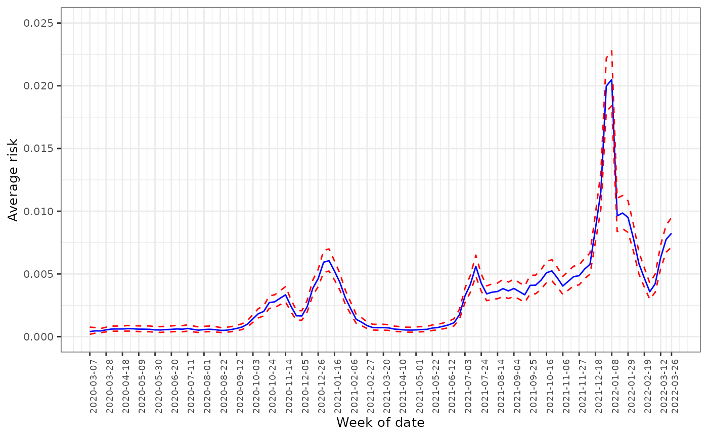
The average predicted infection risk in weeks
Finally, we create a map showing the spatial pattern of the time averaged risks of infection in England.
average_risk_by_nb <-
dplyr::group_by(predictions, MSOA11CD) %>% dplyr::summarize(ave.risk = mean(pred.mean))
sp_data@data$ave.risk <- average_risk_by_nb$ave.risk
domain <- sp_data@data$ave.risk
fdmr::plot_map(
polygon_data = sp_data,
domain = domain,
palette = "Reds",
legend_title = "Risk",
add_scale_bar = TRUE,
polygon_fill_opacity = 1,
polygon_line_colour = "transparent"
)Map of the average predicted infection risks
Evaluate the performance of prediction
Measuring the prediction accuracy of a model is a critical aspect of evaluating its performance, especially in the context of time-series data where new information becomes available over time. To measure the prediction accuracy of the model, a moving time series window of training and validation data was considered when new data comes in throughout the pandemic. This approach allows the model to continuously update its parameters based on the latest available data, rather than relying on a static dataset that may not reflect the current situation. We started with an initial training dataset of 96 weeks from 2020/03/07 to 2022/01/01, and then used this to predict the infection risk for week and all neighbourhoods . The prediction was then compared to the actual observed values to determine the accuracy of the model. This process is repeated for each subsequent week as new data becomes available.
The accuracy of risk prediction is measured by the root mean square error (RMSE), bias and coverage probabilities of the 95% credible intervals for the corresponding risk estimates. RMSE quantifies the average magnitude of the differences between the predicted and the observed values, and a lower value indicates better prediction performance. The of the risk estimates in week over all neighbourhoods is calculated as
where and are the predicted and observed infection risk in neighbourhood and week respectively. is the total number of neighbourhoods with reported COVID infection data in week . Bias measures the average difference between the predicted and the observed values. The bias of the risk predictions of all neighbourhoods in week is calculated as
The uncertainty of the risk predictions can be measured by the coverage probabilities of the 95% credible intervals. The 95% coverage probability (denoted ) is computed as the proportion of the 95% credible intervals for that contain the observed risk.
In addition, to measure the magnitude of the differences between the predicted and observed values in relation to the observed values, the relative root mean square error (R-RMSE) and relative bias (R-Bias) are also computed. The relative root mean square error () is calculated as
The relative bias () is calculated as
As new data comes in every week, all previous data are used for training the model, and the , , , and are updated using new validation data of week . Finally, we create time series of , and over week in , which summarise the progress of the predictive capabilities of the model over time.
The values of
,
,
,
and
for week
in
are stored in the tutorial data package and we’ll load the
data.frame containing that data now.
predmetrics <- fdmr::load_tutorial_data(dataset = "covid", filename = "predmetrics.rds")This figure displays the time series plots for , and . The plots suggest that our model performs well in predicting the rate of COVID-19 infection, because the RMSE and bias values are very low (close to 0) compared to the range of the observed risks, and the coverage probabilities are close to their nominal 0.95 level. Table 3 provides the median and mean values for , , , and for .
breaks_vec <- c(seq(min(predmetrics$date),
max(predmetrics$date),
by = "1 week"
))
RMSEt <- predmetrics[, c("date", "RMSEt")]
Biast <- predmetrics[, c("date", "Biast")]
CPt <- predmetrics[, c("date", "CPt")]
g1 <-
fdmr::plot_timeseries(
data = RMSEt,
# TODO - update these to just accept a string
x = "date",
y = "RMSEt",
breaks = breaks_vec,
x_label = "Date",
y_label = "RMSE",
y_lim = c(0, 0.05),
horizontal_y = 0
)
g2 <-
fdmr::plot_timeseries(
data = Biast,
x = "date",
y = "Biast",
breaks = breaks_vec,
x_label = "Date",
y_label = "Bias",
y_lim = c(-0.01, 0.01),
horizontal_y = 0
)
g3 <-
fdmr::plot_timeseries(
data = CPt,
x = "date",
y = "CPt",
breaks = breaks_vec,
x_label = "Date",
y_label = "Coverage probability",
y_lim = c(0, 1),
horizontal_y = 0.95
)
gridExtra::grid.arrange(g1, g2, g3, nrow = 1)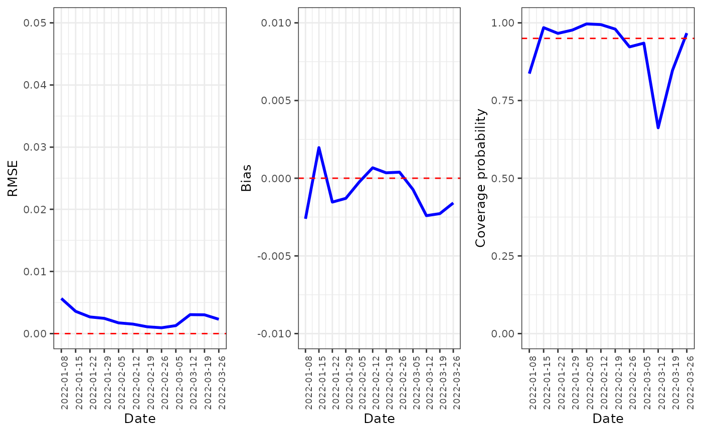
RMSE, bias and coverage probability for the model over time.
| Metric | Median | Mean |
|---|---|---|
| 0.0024 | 0.0024 | |
| -0.0010 | -0.0008 | |
| 0.9665 | 0.9224 | |
| 0.1566 | 0.1553 | |
| -0.1102 | -0.0352 |
Discussion
The study provides valuable insights into the spread and evolution of COVID-19 occurrences at the MSOA level in mainland England from March 7, 2020 to March 26, 2022. It found that there are significant health inequalities in COVID infection across England, with the magnitude of these inequalities appearing to have increased over time, which emphasizes the need for effective strategies to address the disparities in COVID-19 risk between different neighbourhoods. The COVID infection risk in England has fluctuated over time with an overall upward trend, and people appear to be at higher risk of COVID infection in June, July, December, and January, which is likely due to June and July are popular months for travelling, outdoor activities and social gatherings in the UK, and December and January are associated with holiday celebrations (Christmas and New Year’s holiday), family gatherings, and travel. These events often involve close contact with others, which can increase the risk of COVID-19 transmission. Colder and drier conditions during the winter months could also make the COVID-19 virus more transmissible (Mecenas et al. (2020), Wang et al. (2021)). The low estimated infection risks and small variation in the first weeks of the study period is probably due to the limited capacity for COVID-19 testing in the first wave of the pandemic. Testing was only available to priority groups and was not comprehensive, meaning that many infected people were not diagnosed with the virus. This likely led to under-reporting of confirmed COVID-19 cases, which in turn led to low infection rates and small variation.
The results from the model have shown clear evidence that socioeconomic deprivation is positively associated with increased COVID-19 incidence, which aligns with the findings in Oluyomi et al. (2021), Kulu and Dorey (2021) that the virus has hit harder in areas of higher deprivation. This is likely due to individuals living in deprived areas having limited access healthcare facilities and resources, exhibiting higher prevalence of underlying health conditions, and relying more heavily on public transportation, which all contribute to higher infection rates.
Ethnicity was found to have a strong association with COVID-19 infection. Chinese and African populations were found to be associated with lower risk of infections, whereas Indian and Pakistani ethnic groups, Caribbean population, and white British population were associated with higher risk of infections. The lower infection rates in Chinese might be attributed to their greater emphasis on collective responsibility and community health, which have helped to encourage adherence to public health guidelines and prevent the spread of the virus, while white British individuals appear to be less likely to adhere to recommended COVID-19 related health behaviours compared to other ethnic groups https://www.iser.essex.ac.uk/blog/2021/06/14/are-there-ethnic-differences-in-adherence-to-recommended-health-behaviours-related-to-covid-19.
Neighborhoods with a greater percentage of adults aged 65 and older, and those with a greater percentage of adults aged 18-29, were found to have a lower risk of infections, while the populations between 30 and 44 years old, and between 45 and 64 years old, were positively associated with the risk of infections. These findings may be explained from aspects of vaccination rates, lifestyle and health status. For example, older people are among the first groups to be prioritized for COVID-19 vaccination in the UK, leading to lower COVID infection rates. Young adults (aged 18-29) may be more likely to comply with public health guidelines and regulations, such as social distancing and wearing masks, to to avoid exposure to the virus. Additionally, younger adults are more likely to have jobs that allow them to work from home, reducing their exposure to the virus in public spaces. Conversely, middle-aged adults (aged 45-64 years old) may be more likely to work in essential jobs that require them to interact with the public, increasing their exposure to the virus.
Elevated and levels were also found to be positively associated with COVID-19 infections. Exposure to air pollution can cause inflammation and damage to the respiratory system, which may increase susceptibility to respiratory infections such as COVID-19 (Fattorini and Regoli (2020), Comunian et al. (2020)). Air pollution has been shown to worsen underlying health conditions such as diabetes, cardiovascular, and respiratory diseases, which are known risk factors for severe illness from COVID-19 (Semczuk-Kaczmarek et al. (2021)).
It is important to note that the relationship between COVID-19 infection risk and race, age, air pollution and socioeconomic status is complex and multifactorial. While the results showed that the risk factors considered in the study have a well-established relationship with COVID-19 infections, there is not necessarily a causal relationship. More research is needed to understand the mechanisms behind these associations. Nonetheless, these findings suggest that targeted interventions for specific age and race groups may be necessary to control the spread of COVID-19 in different neighborhoods, and reducing air pollution levels could be an important public health intervention for mitigating the spread of COVID-19.
Our analysis has highlighted the associations between COVID-19 infection and a set of socioeconomic, demographic and environmental factors. There are several areas for future work that could further expand our understanding of the spread and evolution of COVID-19. It would be beneficial to extend the study period to include more recent data in order to examine any potential changes in the associations between COVID-19 risk and the various factors identified in the study. The analysis can be extended to examine the impacts of other potential factors, such as comorbidities and COVID-19 vaccination rates, that may contribute to the spread of COVID-19. Including these factors in future studies could provide a more comprehensive understanding of the determinants of COVID-19 risk. Such information is useful for policy makers in determining the most effective strategies for controlling the spread of COVID-19 and reducing health inequalities in England. Finally, it would be important to extend the study to other countries and regions to examine whether the results from this study are generalizable to other settings. This could provide valuable insights into the global spread of COVID-19 and inform the development of more effective strategies and targeted actions for preventing the spread of the virus.