Setting up the R environment
If you do not have INLA or inlabru
installed please check our installation
instructions before continuing. First we load INLA and then download
the data for this tutorial from our data repository using
retrieve_tutorial_data.
library(INLA)## Loading required package: Matrix## This is INLA_25.02.10 built 2025-02-09 19:59:04 UTC.
## - See www.r-inla.org/contact-us for how to get help.
## - List available models/likelihoods/etc with inla.list.models()
## - Use inla.doc(<NAME>) to access documentation
fdmr::retrieve_tutorial_data(dataset = "hydro")##
## Tutorial data extracted to /tmp/RtmpRo1mlh/fdmr/tutorial_data/hydroKvilldal dam area
First we will look at the location of the dam by making a map and plotting the stream gauges on it.
norway_polygon_path <- fdmr::get_tutorial_datapath(dataset = "hydro", filename = "Kvilldal_Catch_Boundary.geojson")
norway_polygon <- sf::read_sf(norway_polygon_path) %>% sf::st_zm()
sfc <- sf::st_transform(norway_polygon, crs = "+proj=longlat +datum=WGS84")
We want to mark the position of the dam and the stream gauges on the
map so we’ll create a data.frame to pass into the
plot_map function with the names and positions. We’ll
create a list for each of the points and then use the
(dplyr::bind_rows)[https://dplyr.tidyverse.org/reference/bind.html]
function to create a data.frame from these.
suldalsvatnet_dam <- list(longitude = 6.517174, latitude = 59.490720, label = "Suldalsvatnet Dam")
stream_gauge_13 <- list(longitude = 6.5395789, latitude = 59.5815849, label = "Stream Gauge 13")
stream_gauge_14 <- list(longitude = 6.7897968, latitude = 59.7531662, label = "Stream Gauge 14")

points <- list(suldalsvatnet_dam, stream_gauge_13, stream_gauge_14)
markers <- dplyr::bind_rows(points)
We’re now ready to plot the map, passing in the polygon data, markers and optionally the fill opacity.
fdmr::plot_map(polygon_data = sfc, markers = markers, polygon_fill_opacity = 0.5)On the map you can see the dam, the resevoir, the catchment area, and the two stream gauges. The area inside the shape is where water accumulates, the area outside of the boundary has water that goes elsewhere. This will be important later when we are including ERA5-land precipitation data.
Stream gauge data
The stream gauge data is measured as the average daily liters/second that pass through the area. This data goes back for many years, sometimes decades, so we’ll take a subset of the data for October 2021.
streamdata_13 <- fdmr::get_tutorial_datapath(dataset = "hydro", filename = "NVEobservations_s36_13.csv")
streamdata_14 <- fdmr::get_tutorial_datapath(dataset = "hydro", filename = "NVEobservations_s36_14.csv")

data_13 <- read.csv(streamdata_13)
data_13$date <- as.Date(data_13$time)
data_13 <-
  subset(data_13, date >= "2021-10-01" & date <= "2021-10-31")
row.names(data_13) <- NULL
data_13$time_index <- seq(1, 31, 1)

data_14 <- read.csv(streamdata_14)
data_14$date <- as.Date(data_14$time)
data_14 <-
  subset(data_14, date >= "2021-10-01" & date <= "2021-10-31")
row.names(data_14) <- NULL
data_14$time_index <- seq(1, 31, 1)
We can now plot the average stream flow using
plot_timeseries
fdmr::plot_timeseries(data = data_13, x = "time", y = "value", x_label = "Time", y_label = "Stream Flow: Daily Average (Liter/s)", line_colour = "violet")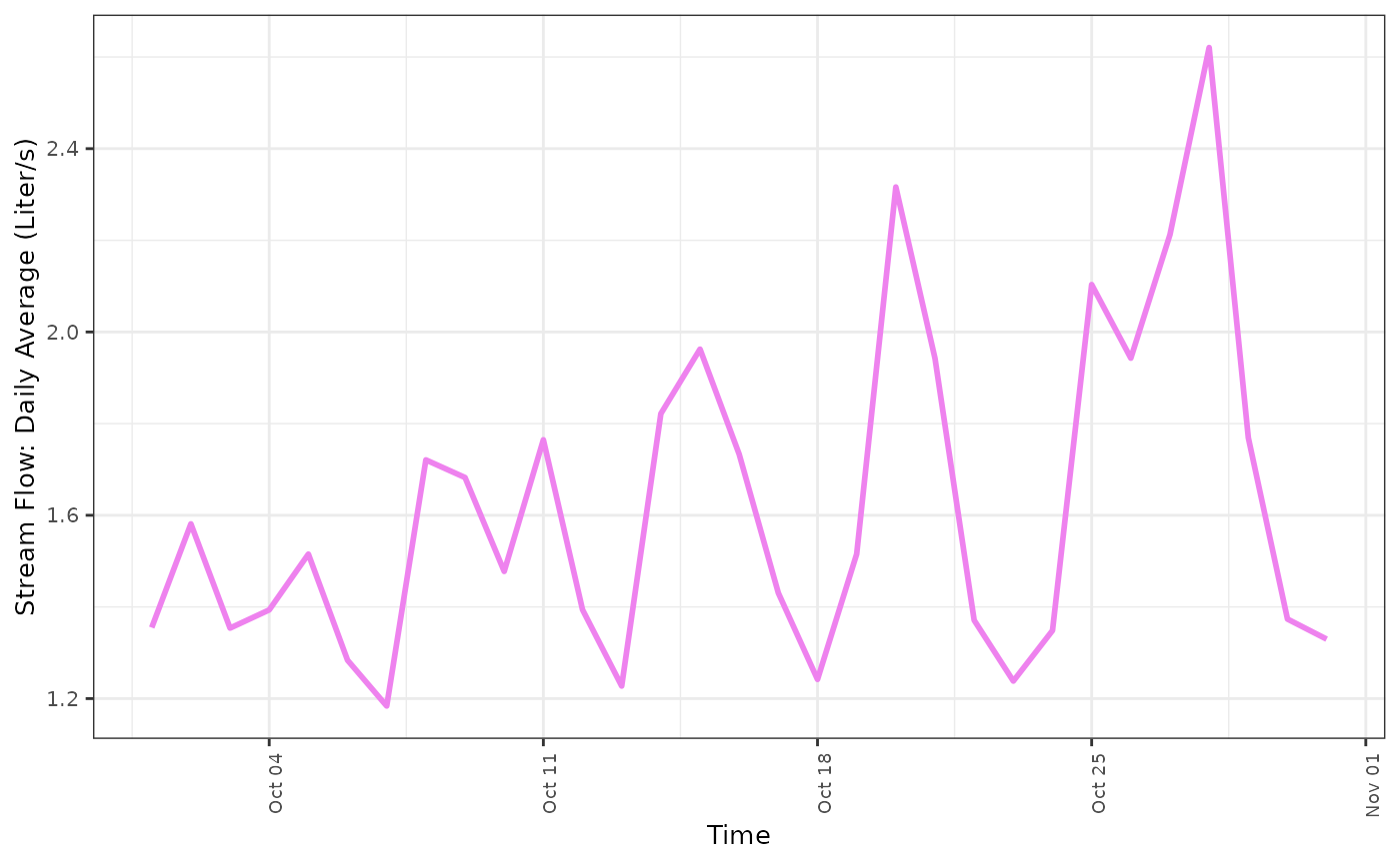
fdmr::plot_timeseries(data = data_14, x = "time", y = "value", x_label = "Time", y_label = "Stream Flow: Daily Average (Liter/s)", line_colour = "limegreen")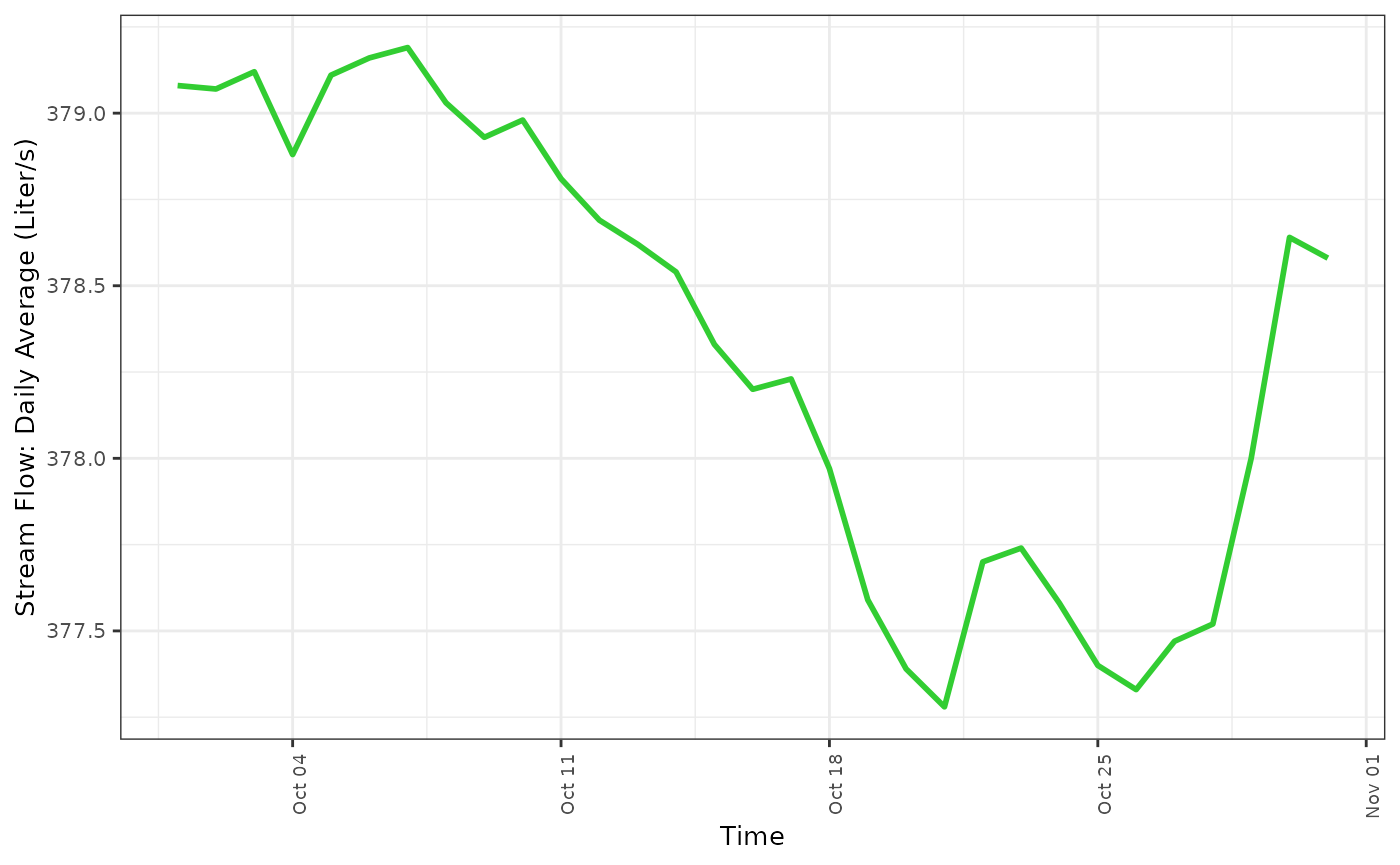
We rescale the data with the Z-score since the values are so different between the two stream gauges
You can see, these two different stream gauges record a very different amount of stream flow. Therefore we should likely normalize this data using the zscore. The response variable in this study is the stream flow measurement. The amount of water that passes through the stream gauge is representative of the amount of water that will accumulate in the resevoir. Thus, in order to understand how this changes over time, it will be important to understand what physical processes drive water into the streams that feed the resevoir.
ERA5-land data
ERA5-land data includes many variables. Here we use only the daily precipitation data. ERA5-land precipitation comes from reanalysis of the climate model. ERA5-land data is gridded however we need the data to be assigned to catchment shapes. We’ll first load in the data, ensure it is projected using the correct coordinate reference system (CRS) and then plot it on a map.
era5_location <- fdmr::get_tutorial_datapath(dataset = "hydro", filename = "era5_land_daily.nc")
era5_precip <- raster::stack(era5_location)
## Loading required namespace: ncdf4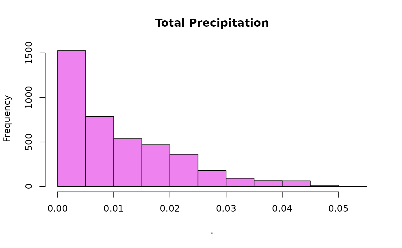
sr <- "+proj=utm +zone=32"
projected_raster <- raster::projectRaster(era5_precip, crs = sr)

era5_precip_cropped <- raster::mask(projected_raster, norway_polygon)
era5_precip_cropped <- terra::crop(era5_precip_cropped, raster::extent(norway_polygon), snap = "near")
Next we create a data.frame raster_df
containing precipitation data. We convert the RasterBrick
of precipitation data we just plotted into a data.frame. We
then want to get only the day component from the date of each date. If
we have a look at the names of each layer in the
RasterBrick you can see that each is prepended with an X,
this is due to raster not allowing layer names that start
with numbers. First we need to remove the X, which we do with
numbers_only. Then we convert the strings to
Date objects using to_dates before finally
using lubridate::day to get just the day component of the
date. Finally, we set the names of the columns in the
data.frame.
raster_df <- data.frame(raster::rasterToPoints(era5_precip_cropped))
raster_df <- data.table::melt(data.table::setDT(raster_df), id.vars = c("x", "y"), variable.name = "time")

raster_df$time <- lubridate::day(fdmr::to_dates(fdmr::numbers_only(raster_df$time)))

raster_df <- setNames(raster_df, c("x", "y", "time", "precip"))
We need to figure out which ERA5 precipitation pixels are closest to which stream gauge so we can match the data for the regression. First we need to calculate the distance between the pixel and each stream gauge, then use the minimum distance to choose the stream gauge. We first convert the lat/long coordinates to UTM and then match the pixel precipation data to the nearest stream gauge.
pixel_coords <- unique(sp::coordinates(era5_precip_cropped))
s13_utm <- fdmr::latlong_to_utm(
  lat = stream_gauge_13$latitude,
  lon = stream_gauge_13$longitude
)
s14_utm <- fdmr::latlong_to_utm(
  lat = stream_gauge_14$latitude,
  lon = stream_gauge_14$longitude
)

s13 <- data.frame(x = s13_utm[[1]], y = s13_utm[[2]])
s14 <- data.frame(x = s14_utm[[1]], y = s14_utm[[2]])

pixel_dist_gauge <- data.frame(
  x = pixel_coords[, 1],
  y = pixel_coords[, 2],
  dist_s1 = rep(NA, nrow(pixel_coords)),
  dist_s2 = rep(NA, nrow(pixel_coords)),
  min_s = rep(NA, nrow(pixel_coords)),
  streamflow = rep(NA, nrow(pixel_coords))
)
for (i in seq_len(nrow(pixel_coords))) {
  pixel_dist_gauge$dist_s1[i] <- sqrt((pixel_dist_gauge$x[i] - s13$x)^2 + (pixel_dist_gauge$y[i] - s13$y)^2)

  pixel_dist_gauge$dist_s2[i] <- sqrt((pixel_dist_gauge$x[i] - s14$x)^2 + (pixel_dist_gauge$y[i] - s14$y)^2)

  pixel_dist_gauge$min_s[i] <- which.min(c(pixel_dist_gauge$dist_s1[i], pixel_dist_gauge$dist_s2[i]))
}
The data.frame pixel_dist_gauge then needs
to be replicated by the number of time points, in this case, layers in
the RasterBrick.
n_time <- raster::nlayers(era5_precip)

pixel_dist_gauge <- do.call(rbind, replicate(n_time, pixel_dist_gauge, simplify = FALSE))
pixel_dist_gauge$time <- rep(1:n_time, each = nrow(pixel_coords))

streamdata <- list(data_13, data_14)

get_stream_data <- function(row) {
  which_stream_data <- streamdata[[row["min_s"]]]
  data_at_row_time_index <- which_stream_data[which_stream_data[, c("time_index")] == row["time"], ]
  return(data_at_row_time_index$value)
}

pixel_dist_gauge$streamflow <- apply(pixel_dist_gauge, 1, get_stream_data)
Now we create a new SpatialPointsDataFrame called
inla_data for model fitting. The data.frame
contains the response and predictor data at each spatial location and
time point.
inla_data <- merge(pixel_dist_gauge, raster_df, by = c("time", "x", "y"))
inla_data <- subset(inla_data, select = c("x", "y", "streamflow", "precip", "time"))

sp::coordinates(inla_data) <- c("x", "y")

head(inla_data@data)
## streamflow precip time
## 1 -0.7379358 0.007305657 1
## 2 -0.7379358 0.006965242 1
## 3 -0.7379358 0.006590370 1
## 4 -0.7379358 0.006557765 1
## 5 -0.7379358 0.007222239 1
## 6 -0.7379358 0.006858168 1
head(inla_data@coords)## x y
## 1 331417.8 6583370
## 2 342677.8 6594470
## 3 348307.8 6594470
## 4 353937.8 6594470
## 5 353937.8 6605570
## 6 359567.8 6594470Creating the BHM using 4D-Modeller
In order to model this with the 4D-Modeller we need to:
- Create a spacial mesh which the SPDE model can be evaluated over
- Build the SPDE model
- Define how the process evolves over time
Mesh resolution
Create the triangulated mesh of the study region and have a quick look at it.
e <- era5_precip_cropped@extent
resolution <- raster::res(era5_precip_cropped)
crs <- "+proj=utm +zone=32"

xres <- resolution[1] * 2
yres <- resolution[2] * 2

xy <- sp::coordinates(era5_precip_cropped)
xy <- xy[seq(1, nrow(xy), by = 2), ]

colnames(xy) <- c("LONG", "LAT")

mesh <- fmesher::fm_mesh_2d_inla(loc = xy, max.edge = c(xres * 1, xres * 100), cutoff = 75, crs = crs)

fdmr::plot_mesh(mesh)
Priors
The priors here are describing how the unobserved variannce is distributed over the region. That is, how far away from the center of the process should it cease to spatially correlate with the surrounding environment. To put it a different way, if it is raining on a hill top, how far from that hill must you be to not notice if it’s raining or not.
In this case, we set the prior range to be 20km.
# prior.range<-0.296
# the prior range is the distance that the process should stop effecting, so in this case it is currently 20km away from the node center
prior_range <- 20.0
spde <- INLA::inla.spde2.pcmatern(
  mesh = mesh,
  prior.range = c(prior_range, 0.5),
  prior.sigma = c(1, 0.01)
)
the model has some time dependency.
In order to fit the model, we also need to define a temporal index and the number of discrete time points we want to model. The INLA model requires that time indicies must be an integer starting at 1.
Model Inference
The model below predicts the streamflow given the precipitation as a fixed effect and an SPDE model which assumes there is some other correlation structure in the streamflow data due to unobserved variables. Likely unobserved co-variates could be local elevation, temperature, soil permeability, or presence of vegetation.
formula1 <- streamflow ~ 0 + Intercept(1) + precip

formula2 <- streamflow ~ 0 + Intercept(1) + precip +
  f(
    main = coordinates,
    model = spde,
    group = time,
    ngroup = n_groups,
    control.group = list(
      model = "ar1",
      hyper = rhoprior
    )
  )
inlabru_model1 <- inlabru::bru(formula1,
  data = inla_data,
  family = "gaussian",
  options = list(
    verbose = FALSE
  )
)

inlabru_model2 <- inlabru::bru(formula2,
  data = inla_data,
  family = "gaussian",
  options = list(
    verbose = FALSE
  )
)
## Warning in handle_problems(e_input): The input evaluation 'coordinates' for 'f'
## failed. Perhaps you need to load the 'sp' package with 'library(sp)'?
## Attempting 'sp::coordinates'.Now it’s time to see its output, we can use the
fdmr::model_viewer and pass in our model output, mesh and
measurement data. This Shiny app helps analyse model output by
automatically creating plots and a map of predictions for your data.
Make sure you have a CRS set on your mesh. If no CRS can be read a
default of "+proj=longlat +datum=WGS84" will be used which
may lead to errors with data using UTM as we’ve done here.
fdmr::model_viewer(model_output = inlabru_model2, mesh = mesh, measurement_data = inla_data, data_distribution = "Gaussian")We can also view the summary of the model outputs
summary(inlabru_model1)## inlabru version: 2.12.0
## INLA version: 25.02.10
## Components:
## Intercept: main = linear(1), group = exchangeable(1L), replicate = iid(1L), NULL
## precip: main = linear(precip), group = exchangeable(1L), replicate = iid(1L), NULL
## Likelihoods:
## Family: 'gaussian'
## Tag: ''
## Data class: 'SpatialPointsDataFrame'
## Response class: 'numeric'
## Predictor: streamflow ~ .
## Used components: effects[Intercept, precip], latent[]
## Time used:
## Pre = 0.378, Running = 0.259, Post = 0.0364, Total = 0.673
## Fixed effects:
## mean sd 0.025quant 0.5quant 0.975quant mode kld
## Intercept -0.248 0.049 -0.343 -0.248 -0.152 -0.248 0
## precip 23.923 3.503 17.052 23.923 30.792 23.923 0
##
## Model hyperparameters:
## mean sd 0.025quant 0.5quant
## Precision for the Gaussian observations 1.09 0.052 0.99 1.09
## 0.975quant mode
## Precision for the Gaussian observations 1.20 1.09
##
## Deviance Information Criterion (DIC) ...............: 2394.72
## Deviance Information Criterion (DIC, saturated) ....: 873.36
## Effective number of parameters .....................: 2.98
##
## Watanabe-Akaike information criterion (WAIC) ...: 2394.28
## Effective number of parameters .................: 2.53
##
## Marginal log-Likelihood: -1215.68
## is computed
## Posterior summaries for the linear predictor and the fitted values are computed
## (Posterior marginals needs also 'control.compute=list(return.marginals.predictor=TRUE)')
summary(inlabru_model2)## inlabru version: 2.12.0
## INLA version: 25.02.10
## Components:
## Intercept: main = linear(1), group = exchangeable(1L), replicate = iid(1L), NULL
## precip: main = linear(precip), group = exchangeable(1L), replicate = iid(1L), NULL
## f: main = spde(coordinates), group = ar1(time), replicate = iid(1L), NULL
## Likelihoods:
## Family: 'gaussian'
## Tag: ''
## Data class: 'SpatialPointsDataFrame'
## Response class: 'numeric'
## Predictor: streamflow ~ .
## Used components: effects[Intercept, precip, f], latent[]
## Time used:
## Pre = 0.358, Running = 77.5, Post = 2.26, Total = 80.1
## Fixed effects:
## mean sd 0.025quant 0.5quant 0.975quant mode kld
## Intercept -0.165 0.301 -0.760 -0.165 0.428 -0.165 0
## precip 14.646 6.163 2.575 14.633 26.795 14.633 0
##
## Random effects:
## Name Model
## f SPDE2 model
##
## Model hyperparameters:
## mean sd 0.025quant 0.5quant
## Precision for the Gaussian observations 3.51e+04 2.83e+04 4454.25 2.73e+04
## Range for f 6.70e+04 3.78e+03 59997.35 6.68e+04
## Stdev for f 8.22e-01 4.90e-02 0.73 8.20e-01
## GroupRho for f 7.28e-01 2.30e-02 0.68 7.29e-01
## 0.975quant mode
## Precision for the Gaussian observations 1.09e+05 1.30e+04
## Range for f 7.49e+04 6.63e+04
## Stdev for f 9.24e-01 8.16e-01
## GroupRho for f 7.71e-01 7.31e-01
##
## Deviance Information Criterion (DIC) ...............: -5591.39
## Deviance Information Criterion (DIC, saturated) ....: 1827.49
## Effective number of parameters .....................: 960.77
##
## Watanabe-Akaike information criterion (WAIC) ...: -5840.68
## Effective number of parameters .................: 538.45
##
## Marginal log-Likelihood: 65.79
## is computed
## Posterior summaries for the linear predictor and the fitted values are computed
## (Posterior marginals needs also 'control.compute=list(return.marginals.predictor=TRUE)')