Simulation Tutorial (Poisson data)

In this tutorial, we’ll start by generating some simulated spatio-temporal data, with the city of Bristol as our study region. Next, we’ll walk you through the steps of running the Bayesian Hierarchical Model (BHM) using the INLA-SPDE approach. Finally, we’ll demonstrate the use the key functionality provided by the fdmr package.

Data simulation

First we simulate some Gaussian distributed data observed at 55 spatial locations in Bristol, UK and across 6 time points. We use the fdmr::retrieve_tutorial_data function and the fdmr::load_tutorial_data function to retrieve and load in the geographical information for the spatial locations in Bristol from the fdmr example data store.

fdmr::retrieve_tutorial_data(dataset = "priors")

## 
## Tutorial data extracted to  /home/runner/fdmr/tutorial_data/priors

sp_data <- fdmr::load_tutorial_data(dataset = "priors", filename = "spatial_dataBris.rds")

Then we simulate the Poisson data that exhibit spatio-temporal correlation. These simulated data are finally organized into a data frame named simdf, where each row corresponds to an observation at a specific location and time. The variable ID is the spatial location identifier. Variable time denotes the time point. The variable datn represents the simulated response data. The variable E is the exposure variable of the Poisson data. The longitude and latitude coordinates for each location are stored in the variables LONG and LAT, respectively.

library(INLA)

## Loading required package: Matrix

## Loading required package: sp

## This is INLA_23.12.17 built 2023-12-17 16:59:33 UTC.
##  - See www.r-inla.org/contact-us for how to get help.
##  - List available models/likelihoods/etc with inla.list.models()
##  - Use inla.doc(<NAME>) to access documentation

library(dplyr)

## 
## Attaching package: 'dplyr'

## The following objects are masked from 'package:stats':
## 
##     filter, lag

## The following objects are masked from 'package:base':
## 
##     intersect, setdiff, setequal, union

n.time <- 6
n <- 55
locs <- as.matrix(sp_data@data[, c("LONG", "LAT")])

initial_range <- diff(range(locs[, 1])) / 3
max_edge <- initial_range / 2
mesh <- fmesher::fm_mesh_2d(
  loc = locs,
  max.edge = c(1, 2) * max_edge,
  offset = c(initial_range, initial_range),
  cutoff = max_edge / 7
)

spde <- INLA::inla.spde2.pcmatern(
  mesh = mesh,
  prior.range = c(initial_range, 0.5),
  prior.sigma = c(1, 0.01)
)


sigma0 <- 100
range0 <- 0.03
kappa0 <- sqrt(8 / 1) / range0
tau0 <- 1 / (sqrt(4 * pi) * kappa0 * sigma0)
inla.seed <- sample.int(n = 1E4, size = n.time)
Q <- INLA::inla.spde.precision(spde, theta = c(log(tau0), log(kappa0)))
x.mat <- matrix(NA, ncol = n.time, nrow = mesh$n)
for (co in 1:ncol(x.mat)) {
  x.mat[, co] <- INLA::inla.qsample(n = 1, Q)
}

A <- INLA::inla.spde.make.A(mesh = mesh, loc = locs)
x.dat <- matrix(NA, ncol = n.time, nrow = n)
for (t in 1:ncol(x.dat)) {
  x.dat[, t] <- drop(A %*% x.mat[, t])
}


alpha <- 0.9
sp.mat <- matrix(NA, ncol = n.time, nrow = n)
sp.mat[, 1] <- x.dat[, 1]
for (t in 2:n.time) {
  sp.mat[, t] <- alpha * sp.mat[, t - 1] + x.dat[, t]
}

beta0 <- 0.5
sigma_e <- 0.1
lin.pred <- beta0 + sp.mat + matrix(rnorm(n * n.time, 0, sigma_e), ncol = n.time)

E.mat <- matrix(rep(sample(20:50, n, replace = TRUE), n.time), ncol = n.time)
lambda <- E.mat * exp(lin.pred)
y.mat <- matrix(NA, ncol = n.time, nrow = n)
for (t in 1:n.time) {
  y.mat[, t] <- rpois(n, lambda = lambda[, t])
}

simdf <- data.frame(
  ID = rep(1:n, each = n.time),
  time = rep(c(1:n.time), n),
  datn = as.numeric(t(y.mat)),
  E = as.numeric(t(E.mat)),
  LONG = rep(locs[, 1], each = n.time),
  LAT = rep(locs[, 2], each = n.time)
)

A histogram is created to visualize the distribution of the simulated data.

hist(simdf$datn, main = "", xlab = "Data")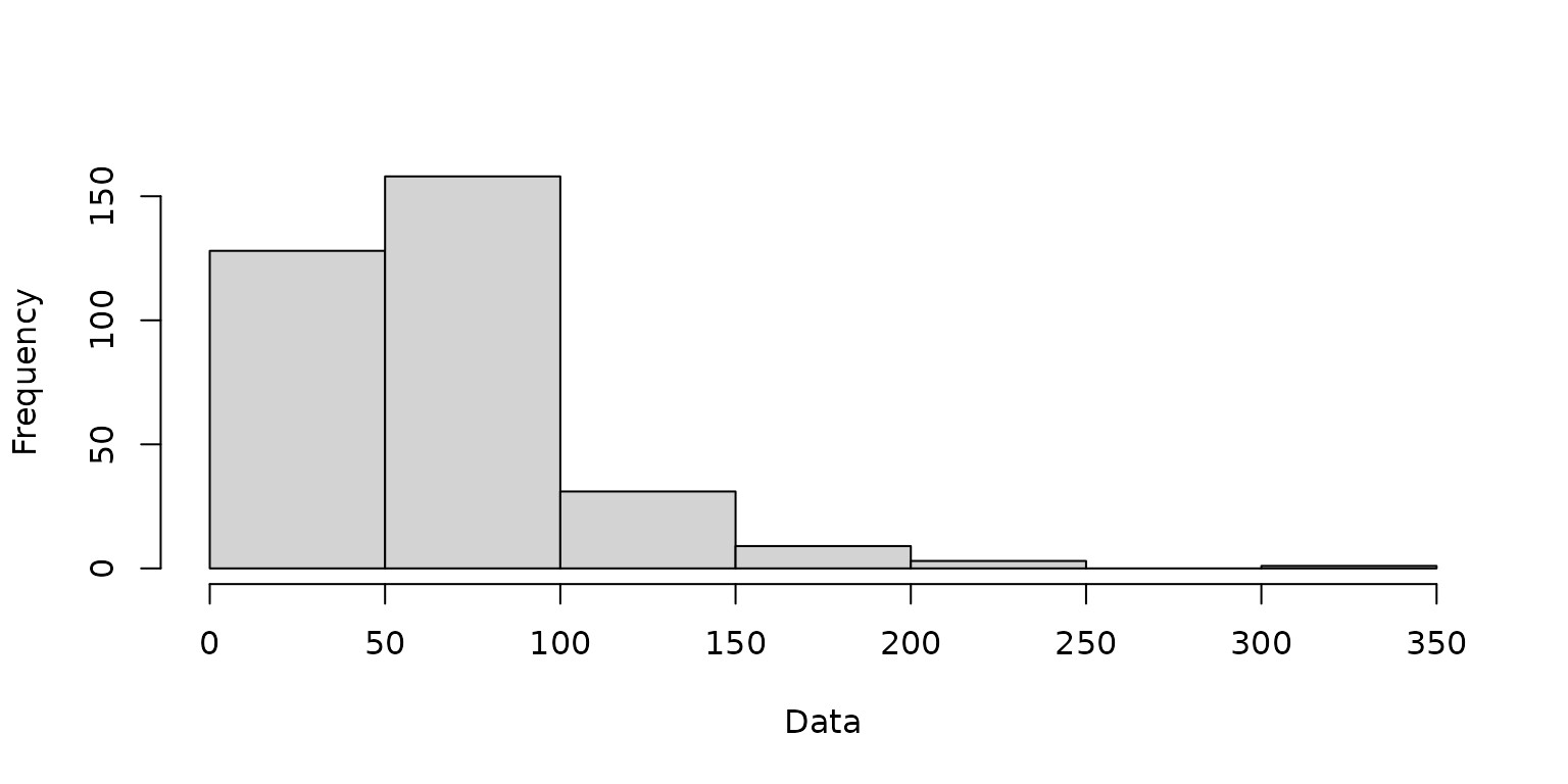

A histogram of the simulated Poisson data.

We can also map the simulated data using the fdmr::plot_map function. .

dat_by_ID <- dplyr::group_by(simdf, ID) %>% dplyr::summarize(sum.dat = sum(datn))
fdmr::plot_map(
  polygon_data = sp_data,
  domain = dat_by_ID$sum.dat,
  palette = "Reds",
  legend_title = "Data",
  add_scale_bar = TRUE,
  polygon_fill_opacity = 1,
  polygon_line_colour = "transparent"
)

A map of the simulated data in Bristol over all time periods.

Model fitting

With the simulation dataset now prepared, our next step is to implement a Bayesian spatio-temporal model using the INLA-SPDE approach.

Generate mesh, build the SPDE model, and set priors for the spatial parameters

locs <- unique(simdf[, c("LONG", "LAT")])
initial_range <- diff(range(locs[, 1])) / 3
max_edge <- initial_range / 2
mesh <- fmesher::fm_mesh_2d(
  loc = locs,
  max.edge = c(1, 2) * max_edge,
  offset = c(initial_range, initial_range),
  cutoff = max_edge / 5
)

spde <- INLA::inla.spde2.pcmatern(
  mesh = mesh,
  prior.range = c(initial_range, 0.5),
  prior.sigma = c(1, 0.01)
)

Define how the process evolves over time, set prior for the temporal parameter and define a temporal index

rhoprior <- base::list(theta = list(prior = "pccor1", param = c(0, 0.9)))
group.index <- simdf$time
n_groups <- length(unique(simdf$time))

We will use the function bru() of package inlabru to fit the model. bru expects the coordinates of the data, thus we transform simdf data set to a SpatialPointsDataFrame using the function coordinates() of the sp package.

sp::coordinates(simdf) <- c("LONG", "LAT")

Define the model formula

formula <- datn ~ 0 + Intercept(1) +
  f(
    main = coordinates,
    model = spde,
    group = group.index,
    ngroup = n_groups,
    control.group = list(
      model = "ar1",
      hyper = rhoprior
    )
  )

Fit the model

Finally, we fit the spatio-temporal model using SPDE approach and AR(1) process by calling the function bru() of the package inlabru.

inlabru_model <- inlabru::bru(formula,
  data = simdf,
  family = "poisson",
  E = simdf$E,
  control.family = list(link = "log"),
  options = list(
    verbose = FALSE
  )
)

## Warning in inla.model.properties.generic(inla.trim.family(model), mm[names(mm) == : Model 'scopy' in section 'latent' is marked as 'experimental'; changes may appear at any time.
##   Use this model with extra care!!! Further warnings are disabled.

Results summary

After completing the model fitting process, you can examine the main result summaries by typing summary(inlabru_model). Additionally, you can check the parameter estimates for fixed effects, random effects, and hyperparameters as follows.

model_summary <- summary(inlabru_model)
model_fixed <- inlabru_model$summary.fixed
model_random <- inlabru_model$summary.random
model_hyperparams <- inlabru_model$summary.hyperpar

The Deviance Information Criterion (DIC) value, which measures the goodness of model fit, can be examined as follows.

model_dic <- inlabru_model$dic$dic

You can obtain the model’s fitted values and compare them with the observed values as follows.

fitted_vals <- inlabru_model$summary.fitted.values[1:nrow(simdf), ]

par(pty = "s")
plot(fitted_vals$mean, simdf$datn / simdf$E, xlab = "fitted", ylab = "observed")

A plot of the fitted and observed values.

Exploring the functionality of the fdmr Package

Next, we’ll demonstrate the key functionality offered by the fdmr package.

fdmr::plot_mesh

The fdmr::plot_mesh function displays both the mesh and the observation points overlaid on the mesh.

fdmr::plot_mesh(mesh = mesh, spatial_data = simdf@coords)

## Warning in fdmr::plot_mesh(mesh = mesh, spatial_data = simdf@coords): Cannot
## read CRS from mesh, assuming WGS84

## Warning in fdmr::plot_mesh(mesh = mesh, spatial_data = simdf@coords):
## Attempting to convert to a data.frame

A plot of the mesh.

fdmr::mesh_builder

fdmr provides an interactive mesh builder tool called fdmr::mesh_builder. It allows you to build a mesh from some spatial data, modify its parameters and plot it and the data on an interactive map. To build a mesh, we need to pass sp_data to the mesh_builder function.

fdmr::mesh_builder(spatial_data = sp_data)

The interactive map allows you to customise the initial parameters such as max_edge, offset and cutoff to change the shape and size of the mesh.

Model builder Shiny app

fdmr provides a Priors Shiny app which allows you to interactively set and see the model fitting results of different priors. You can launch this app by passing the spatial and observation data to the fdmr::model_builder function.

fdmr::model_builder(
  spatial_data = sp_data,
  measurement_data = simdf,
  mesh = mesh,
  time_variable = "time"
)

On the app interface, you can start by choosing the variable to model. In this example we’ll select datn, then select E for the exposure parameter, and the features to add to the formula. At the bottom of the window you’ll see the formula being constructed. On the left side, you can change the priors for the model parameters. Click on the checkboxes to select your formula and then click the Run Model button to run the model see it’s output plot on the right of the window.

fdmr::model_viewer

fdmr provides a separate Shiny app which allows you to intuitively visualize the model output. You can launch this app by passing the bru model object, the mesh, observation data and data distribution as arguments to the fdmr::model_viewer function.

fdmr::model_viewer(
  model_output = inlabru_model,
  mesh = mesh,
  measurement_data = simdf,
  data_distribution = "Poisson"
)

fdmr::plot_map

The fdmr::plot_map function generates a map of the region based on the provided SpatialPolygonDataFrame.

fdmr::plot_map(polygon_data = sp_data)

A map of the study region.